A Deep Dive Into Vectorfield Pathfinding

Introduction.

Back in 2016, while building a clone of Tanks!, I ran into my first pathfinding challenge. I needed a way for multiple enemy tanks to chase the player around while dodging walls. After digging into the topic, I came across goal-based vector pathfinding (or simply Vector Field Pathfinding - VFP).

It did exactly what I needed, but in a way that felt more visual & intuitive than or Dijkstra. I liked it so much that I even made a video about it in 2020 just to share how cool and practical this approach really is.

The video ended up doing very well for a niche subject! It sparked a lot of great discussions in the comments: people sharing alternative approaches, asking smart questions, or diving deeper into the method.

But looking back, my younger self definitely made a few mistakes. There were some unverified claims, oversimplified explanations, and a lot I just didn’t know back then. More than six years later, I finally decided to revisit this topic, something I’d been wanting to do for a long time, especially as the comments kept rolling in over the years.

This is what this post is about: A Deep dive into Vector Field Pathfinding.
How it works, the many ways you can build and tweak it to fit different needs and where it fits in the spectrum of pathfinding algorithms.

What is pathfinding ?

Before jumping straight into VFP (Vector Field Pathfinding), it’s worth taking a moment to remind ourselves what pathfinding really is ? — where it comes from, and why it exists in the first place.

Defining the problem (a bit of graph theory) :

At its core, pathfinding is a graph theory problem. A graph consists of a set of vertices connected by a set of edges (ie. pairs of vertices). Graphs can also be weighted, meaning each edge has an associated value (or weight) that can represent a distance, a cost, or any other metrics.

The graph representation of

We can thus define pathfinding as finding the shortest path between two vertices of a graph, or more precisely the path between two vertices of a graph such that the sum of the weights of its constituent edges is minimized.

Hover to reveal the shortest path

Setting-up our pathfinding environment :

In this post, we’ll explore a specific type of graph: the 8-neighbor grid graph, (also known as a King’s graph). We can think of it as a 2D grid where each tile connects to all its 8 surrounding neighbors, like how a king moves in chess.

This graph is undirected, meaning connections flow both ways between tiles and each connection (edge) carries a weight determined by a distance kernel—a predefined matrix that might, for instance, make diagonal connections less costly than horizontal or vertical ones.

A 2D Grid w/ its corresponding node graph

Click & Drag over the grid to add walls

With our 2D grid in place, we can now define which tiles are walkable and which act as walls. In graph terms, walkable tiles stay as nodes while walls are simply removed from the graph entirely.

Why are we doing this ?

The 8-neighbor grid graph approach provides a universal way to discretize any 2D space and apply pathfinding —whether for robotic, video games, etc… Therefore finding the shortest path between two tiles while avoiding walls becomes finding the shortest path between two vertices in our modified graph.

Overview of Djikstra algorithm

If you are already familiar with classic pathfinding algorithm, you can skip directly to the VFP implementation. If not, it’s helpful to review one of the most well-known and foundational pathfinding algorithms: Dijkstra’s algorithm.

Understanding how Dijkstra’s algorithm works provides a solid framework for the general steps involved in any pathfinding method. VFP builds directly from these steps, which is why we begin our study here. Similarly, algorithms like also extend Dijkstra’s approach, though they serve different purposes.

Initialisation

The algorithm starts by preparing each node :

All nodes are given a tentative distance to the starting node of infinity (ie. ), reflecting that we don’t yet know how to reach them.
Their previous node value is also initialized to (ie. ), this will let us retrace the shortest path later.
The starting node (or source) is given a distance of , since it’s the point of origin.

Afterward, all nodes are placed in a set , which represents the pool of nodes we still need to process.

Pseudo Code

Main loop

The main loop runs as long as there are nodes in , the set of unvisited nodes. This ensures that we eventually visit all nodes in the graph, allowing us to compute the shortest path from the source to every other node. Intuitively, this loop mimics the spreading of information outward from the source.

Pseudo Code

At each iteration, we select the node with the smallest tentative distance (ie. the most promising frontier) and examine its neighbors. Choosing the closest node first ensures that the search expands gradually across the graph, like a wave, refining distance estimates as it reaches new areas.

The selected node is then removed from , marking it as processed.

Neighbor Evaluation & Distance Update (Relaxation)

For the selected node u, we look at each of its neighbors and we calculate a new tentative distance for each of them. If is shorter than , we update it: this is the relaxation step. At the same time, we record as the previous node that leads to on the current best-known path.

Pseudo Code

This process essentially spreads a “wavefront” of shortest distances to the source across the graph, updating nodes as more efficient paths are discovered.

When the algorithm finishes, each node stores its distance to the target and the next neighbor to reach it. To find the shortest path from any node, simply follow these neighbors step by step until you reach the target.

Details & Implementation tips

Many different implementations of the Djikstra Algorithm exist. I chose this one since it’s one of the simplest to understand, especially for grid-based pathfinding. More efficient implementations exist such as using a binary heap to improve time complexity, particularly for sparse graphs.

Note also that this version runs until all nodes are visited. In practice, if you only need the path to a target node, you can stop once it’s reached. Also instead of initializing the queue with all nodes, another common approach is to start with only the source node and add neighbors to the queue as they are discovered.

How to construct VFP

As mentioned earlier, vectorfield pathfinding builds directly on the Dijkstra algorithm. It reuses the two fundamental steps of Dijkstra’s method to perform pathfinding on a grid or graph with obstacles:

Generate a distance heatmap of the grid — that is, assign to each tile the length of the shortest path to the target node.
Reconstruct the shortest path from any tile by following this distance information.

The key innovation in VFP lies in how the second step is interpreted. Instead of tracing paths explicitly, the algorithm assigns a vector (a 2D arrow) to each tile, pointing in the direction of the next step along the shortest path toward the target. This results in a “vector field” that intuitively guides movement across the grid.

Step 1 : Building the distance heatmap :

Using the Djisktra algorithm :

One way to build VFP’s heatmap is to use a modified version of Dijkstra’s algorithm that propagates distance values outward from the target node, taking walls or obstacles into account. However, unlike the original Dijkstra algorithm, this version doesn’t store the previous node for each tile, since we don’t need to explicitly reconstruct paths.

Each tile is colored by its distance to the cursor. Click & drag mouse to add or remove walls.

Distance Kernel

Color Mode

Show Distance

We can visually represent this heatmap by assigning a given color to a tile, determined by the “real-distance” of this tile to the target as you can see with the animation above.

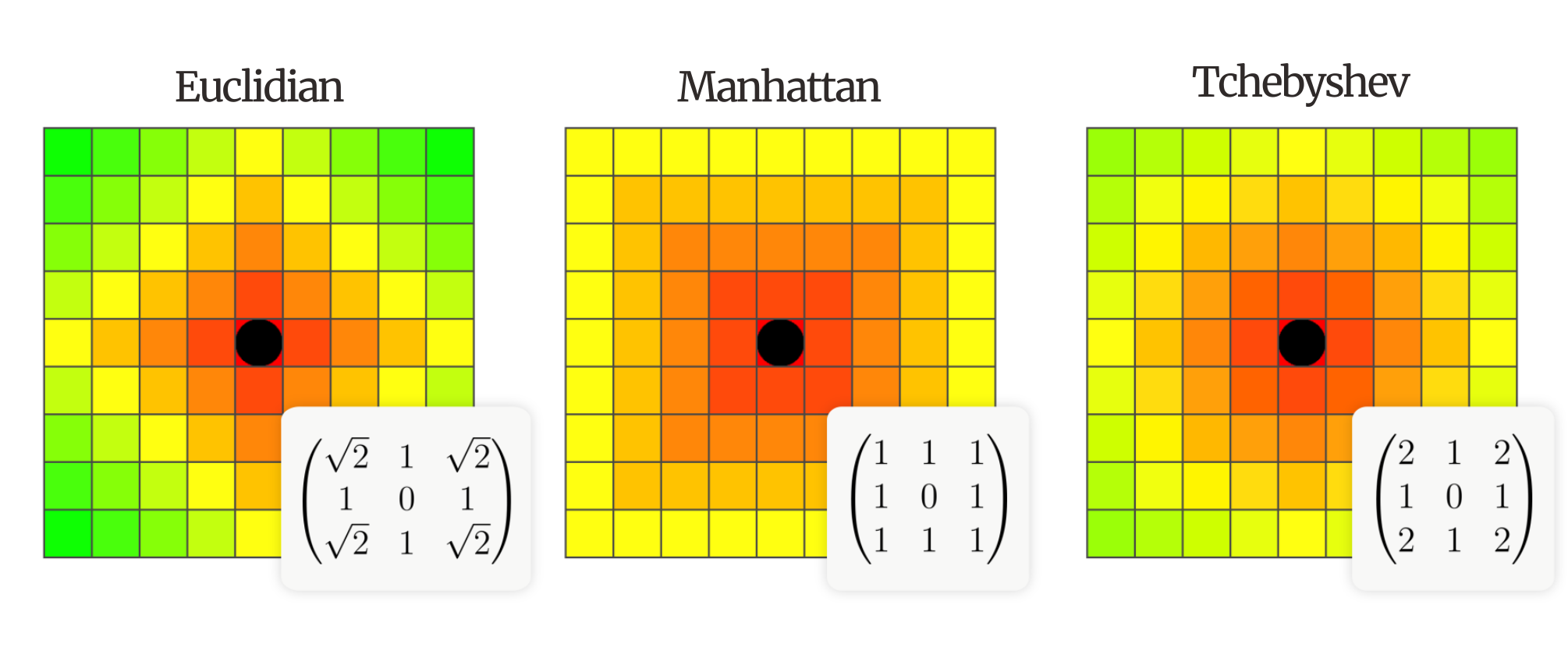
One important customization at this stage involves the choice of distance kernel. As mentioned earlier, the distances between a node and its eight neighbors are determined by a kernel or weight matrix. By selecting different distance matrices, we can control how distances are accumulated, which directly affects the shape of the heatmap and thus the resulting behavior of the pathfinding.

Using the Eikonal equation :

Another way to obtain the distance heatmap of a given 2D grid populated with walls is by solving the Eikonal Equation. Back in 2016, I was unaware of this method but I now found it so elegant and intuitive that I had to share it.

This animation visualizes the propagating wavefront generated by the solution to the Eikonal equation.

Animation Progress

Utility

For a bit of context the Eikonal equation is originally a non-linear PDE that helps models how a wavefront propagates through a medium with varying properties. Intuitively we can think of it as the equation that computes the shortest travel time or minimum distance from a source point to every other point in a domain, taking into account varying speeds or costs throughout the space.

It answers the fundamental question: “What’s the fastest way to get from here to there?”.

Full explanation — Eikonal Equation

The Eikonal equation is :

Where :

is the travel time function (what we seek)
is the speed function (how fast you can travel at position )
is the magnitude of the gradient of

In our case, we define the source by setting the initial condition: ,
And the speed function as follows:

if the node is a wall (i.e., not walkable)
if the node is walkable

With these settings, computing the distance heatmap reduces to solving the Eikonal equation over the grid domain. To do this efficiently, we can use a numerical solver like the Fast Sweeping Method (FSM).

Each tile is colored by its distance to the cursor. Click & drag mouse to add or remove walls.

Color Mode

Show Distance

The eikonal equation offers a continuous alternative to Dijkstra’s algorithm for heatmap generation though it’s originally from a different field and wasn’t designed for graph problems.

What’s the difference with Djikstra

Because it’s continuous, the eikonal solver spontaneously produces smooth, floating-point distance values, unlike Dijkstra, which gives discrete steps. In the eikonal model, the wavefront spreads out in a circular pattern, like a ripple in water.

In contrast, Dijkstra’s wavefront can look square, diamond-shaped, or roughly round depending on the distance kernel used. This makes the eikonal approach appealing: it gives a more natural, physics-inspired result with smoother, more organic heatmaps and fewer artifacts compared to Dijkstra-based methods.

Step 2 : Building the vectorfield :

It’s now time to build the vectorfield: the map that assigns to each grid cell a direction pointing toward the shortest path to the target. In other words, it tells an agent standing on any tile which way to go to reach the goal as quickly as possible.

But how do we compute the vector field from the distance heatmap? The key lies in computing the gradient of the heatmap.

Since our heatmap is defined over a 2D grid, computing its gradient gives us a 2D vector at each point. This vector describes how fast and in which direction the heatmap’s values increase around that point — in other words, the direction of steepest ascent.

And because the heatmap stores distances to the target, following the opposite of the gradient leads along the fastest decrease in distance, meaning the shortest path to the target. So by simply following these vectors, an agent can continuously make locally optimal decisions that guide it along a globally efficient route.

Using the Sobel-operator :

One effective way to compute the gradient of the distance heatmap (and thus derive the vector field) is to use a classic computer vision tool : Sobel operators

It highlights regions with sharp changes in intensity, which correspond to areas with a strong gradient. While its original purpose is edge detection, we can repurpose it here to estimate the gradient across the grid.

Full explanation — Sobel Operator

The Sobel operator consists of two small convolution kernels (or matrices): one estimates the gradient in the x-direction, and the other in the y-direction. When we apply these filters to our heatmap (which is just a 2D grid of values), we obtain for each tile two values:

: the local rate of change in the horizontal direction,
: the local rate of change in the vertical direction.

These two components together define the gradient vector at that point. Now, to extract the orientation of the gradient, we use the arctangent function :

This gives us the angle , which represents the direction in which the heatmap increases the fastest. But our goal is to reach the target, which lies in the direction where the distance decreases the fastest. So, we simply flip the direction by adding :

From this angle, we can easily construct a unit vector (i.e., a vector of length 1) pointing in that direction :

Each tile is colored by its distance to the cursor. Click & drag mouse to add or remove walls.

Using the minDistance neighbor direction :

A simpler method to derive the vectorfield relies on a straightforward observation : the next step toward the goal is always the neighbor with the lowest distance value.

Here’s how it works :

For each tile on the grid, look at its 8-connected neighbors (those directly adjacent in all directions, including diagonals).
Find the neighbor with the lowest distance value on the heatmap, that is, the one closest to the goal.
Draw a vector from the current tile to that neighbor. This vector becomes the local direction for that tile in the vectorfield.

When we move toward the neighbor with the smallest distance, we’re essentially making the locally steepest step down the distance heatmap (a discrete approximation of following the negative gradient).

Important Observation

If you use Dijkstra to build the heatmap, the vectorfield is actually a “free” byproduct.

Instead of deriving directions via convolution, you simply reuse the parent pointers recorded during the search (we actually skip this step in our current djikstra heatmap generation. It should be reimplemented). Since Dijkstra already identifies the optimal neighbor for every node, those pointers are the vector field—no extra math required.

Each tile is colored by its distance to the cursor. Click & drag mouse to add or remove walls.

Using the function weighted neighbor method :

While working on VFP, I found the “minimum neighbor” approach too rigid since it only allows movement in 8 fixed directions. To fix this lack of smoothness, I used an alternative I call the function weighted neighbor :

Full explanation — Weighted Neighbor Sum

For a tile at position p, let = {, …, } be its eight neighbors. For each neighbor pᵢ, define the unit direction:

and let φ(pᵢ) be its distance value.

Each neighbor gets a weight based on how close it is to the goal, using any decreasing function like:

The lower the distance value, the higher the weight.
The smooth direction at p is then:

Instead of picking the single best neighbor, we blend all neighbor directions together, giving more pull to those closer to the goal. Normalizing the sum gives a smooth unit vector that avoids the snapping artifacts of a greedy approach. It essentially approximates the opposite of the distance gradient, pointing toward the steepest descent.

Each tile is colored by its distance to the cursor. Click & drag mouse to add or remove walls.

Weight Function

Agent Motion Over Vectorfield

Once the vector field has been computed, guiding an agent becomes straightforward. The grid contains a 2D vector for each tile that points toward the goal. At each frame, the agent reads the vector beneath its feet and uses it to update its position.

The agent’s motion equation is:

Where:

is the agent’s current position (a 2D vector),
is the agent’s next position,
maps to the grid-tile under the agent,
is the normalized vector stored in the tile ,
is a scalar representing the agent’s speed per time step.

This yields basic motion that aligns the agent with the vector field.

Velocity Smoothing with LERP

To avoid jittery or abrupt changes in direction when crossing from one tile to another, you can smooth the velocity using linear interpolation (LERP). Instead of directly applying the grid vector as velocity, define a target velocity and smoothly interpolate toward it:

Where controls smoothing — low yields slower turning, high makes the agent more responsive.

Each tile is colored by its distance to the cursor. Click & drag mouse to add or remove walls.

Motion Type

Agent Speed

2.0

Particles

LERP Alpha

0.15

Local Limitations and Edge Cases in VFP Computation

When computing the vectorfield, two major types of edge cases arise: grid boundaries and walls in neighbor positions. Both situations present the same core issue: some of the 8-connected neighbors used to compute a vector may either be out of bounds or non-walkable. This becomes especially problematic when using methods like Sobel gradient or weighted neighbor vector summation, which depend on aggregating information from all neighbors.

The difficulty is that walls and out-of-bound cells either lack a meaningful distance value or distort the local gradient. Ignoring them leads to undefined behavior (e.g., division by zero or null vectors), and assigning them arbitrary values often causes the resulting vector to point toward or outward the wall or grid edge. This may lead to path-following artifacts like jitter, backtracking, or agents getting stuck in corners.

A practical fallback solution, although not theoretically grounded at first glance, is to assign out-of-bound or wall neighbors the same distance value as the current node. This flattens the local gradient and avoids introducing artificial directionality. Intuitively, it creates a “neutral slope” at the problematic boundary, allowing surrounding vectors to guide the direction. The resulting vectorfield is smoother, naturally diverges from impassable walls and edges, and helps agents follow walls or slide along boundaries without getting trapped.

Alternatively, a more robust approach is to use the minNeighbor method for these edge cases. Since it doesn’t compute a weighted sum or derivative, but instead selects the neighbor with the lowest distance and points toward it, it handles walls and out-of-bounds naturally: any invalid neighbor is simply excluded from consideration. This ensures correctness without the need for fallback values. Since the method only looks at valid neighbors, it’s inherently more resistant to edge distortions and works well for tiles bordering walls or edges.

Create your custom VFP

Interactive Sandbox: Configure the simulation to your liking using the controls below.

Heatmap

Vector Field

Fallback

Color

Mode

Dist Val

Particles

MOT

SPD 2.0

NUM 10

ALPHA 0.15

Performance, Time Complexity & Common Questions

Now that we’ve covered how VFP works in detail, it’s worth stepping back and asking: where does it actually fit in the landscape of pathfinding? The comment section of my original video surfaced that question repeatedly — along with a few misconceptions I was responsible for spreading. Here are the ones that came up most often, with the answers I should have given back then.

Isn’t VFP just Dijkstra ?

In a some sense, yes, and we’ve already seen why. Dijkstra is the backbone of VFP’s heatmap generation, and with the min-neighbor approach, the vectorfield is essentially a free byproduct: the parent pointers recorded during the search are the vector field, with no extra computation needed.

But the distinction lies in purpose. Dijkstra is a shortest-path algorithm, it finds the optimal route from one node to one target. VFP is a movement model, it precomputes a direction for every tile in the grid, so that any number of agents can navigate toward the goal at near-zero per-agent cost.

Vectorfield pathfinding is not a better shortest-path algorithm than Dijkstra. It’s a better movement architecture for many agents sharing the same goal.

The grid is a choice, not a necessity (and one that I didn’t justify in my original video), mostly because I lacked the theoretical context at the time. Continuous space, navigation meshes, and Voronoi diagrams are all legitimate ways to discretize an environment, and each comes with its own trade-offs.

Grids are popular for this kind of application because they combine simplicity, cache-friendliness, and excellent GPU parallelism. Every tile is the same size, storage is compact, and operations like convolution map perfectly fits to GPU hardware For real-time simulations with large agent counts, those properties will matter a lot.

Is VFP faster than Djikstra / A*?

This was the biggest claim I got wrong in my original video (partly because I wasn’t yet comfortable with complexity analysis, and partly because I simply didn’t verify it).

The honest answer is: it depends on what you’re measuring, and for whom.

First, it’s worth noting that VFP and Djikstra / A* don’t solve quite the same problem. The laters find the shortest path from one specific source to one specific target. VFP builds a complete vector field over the entire grid pointing every tile toward the goal. By design, VFP over-computes when only one agent needs a path.

For a single agent, Djikstra / A* is almost always faster. Especially for A* with its heuristic focuses the search and avoids visiting most of the grid. VFP can’t compete here.

VFP’s advantage emerges when many agents share the same goal. The heatmap and vector field are computed once, then reused by every agent at effectively zero cost per frame : each agent simply reads the vector stored in its current tile.

Beyond that, it’s also worth being clear on path quality: VFP does not guarantee the shortest path. Dijkstra and A* produce topologically optimal paths, but the gradient-based smoothing steps (Sobel, Weighted sum) distort those paths in exchange for geometric smoothness. The only VFP variant that preserves true shortest paths is Dijkstra + min-neighbor, since it reuses the parent pointers directly.

With those nuances in mind, let’s look at how the different algorithms compare in practice. Our context is 2D grid of size tiles.

On the CPU, VFP always performs at least as much work as a plain Dijkstra, since the vector field step is an extra pass over the grid. The exception, again, is the Dijkstra + min-neighbor combination, where the parent pointers double as the vector field at no added cost.

For every other vector field method (Sobel, weighted sum), an additional convolution pass is added on top of whichever heatmap method was used.

Step	Algorithm	Complexity
Heatmap	Dijkstra (naive)
Heatmap	Dijkstra (binary heap)
Heatmap	Eikonal — Fast Marching Method
Heatmap	Eikonal — Fast Sweeping Method	(k = iterations)
Vector Field	Min-neighbor (from Dijkstra parent pointers)	— free byproduct
Vector Field	Sobel operator
Vector Field	Min-neighbor (standalone pass)
Vector Field	Weighted neighbor sum

The GPU picture is quite different and this is where VFP genuinely shines.

Dijkstra is an inherently sequential algorithm: each step depends on the previous one, which makes it a poor fit for GPU parallelism. Note that parallel variants exist (like Parallel BFS), but they generally sacrifice the optimality guarantees of the original.

The Eikonal equation, on the other hand, is better designed for this kind of distributed computation. Methods like the Fast Iterative Algorithm (FIA) decompose the problem into independent local updates that can be dispatched across thousands of GPU threads simultaneously, making full use of SIMD instructions and shared memory.

Convolution (ie. the basis of Sobel, min-neighbor, and weighted sum) is embarrassingly parallel: every tile can be updated independently. On a GPU with threads, an convolution reduces to , which in theory approaches for large grids with enough parallelism.

Step	Algorithm	Complexity
Heatmap	Dijkstra	— poor fit, inherently sequential
Heatmap	Eikonal — Fast Iterative Algorithm	avg. (p = threads)
Vector Field	Sobel operator	→
Vector Field	Min-neighbor	→
Vector Field	Weighted neighbor sum	→

So on the CPU, VFP adds overhead compared to a bare Dijkstra, unless you use the parent-pointer trick to skip the vector field step entirely. On the GPU, the Eikonal + convolution pipeline scales nearly linearly with the number of threads, and on modern hardware that means computing the full vector field for an enormous grid in milliseconds.

So What’s Next ?

One interesting aspect of VFP is that, in the end, it produces an actual vector field that we can explore mathematically. Even if obstacles create undefined regions in the field, methods could be designed to reconstruct or complete those areas.

This opens the door to many possible experiments and extensions. For instance, computing the divergence and curl of the field could help analyze how paths behave locally, such as identifying areas with strong curvature or convergence. Another idea worth exploring would be applying a discrete Helmholtz–Hodge decomposition to better understand and customize the behavior of the generated field.

These are just a few examples of directions that could be explored further by anyone interested in pushing the subject beyond the basics !

A Deep Dive Into Vectorfield Pathfinding

Introduction.

What is pathfinding ?

Defining the problem (a bit of graph theory) :

Setting-up our pathfinding environment :

Overview of Djikstra algorithm

Initialisation

Main loop

Neighbor Evaluation & Distance Update (Relaxation)

How to construct VFP

Step 1 : Building the distance heatmap :

Using the Djisktra algorithm :

Using the Eikonal equation :

Step 2 : Building the vectorfield :

Using the Sobel-operator :

Using the minDistance neighbor direction :

Using the function weighted neighbor method :

Agent Motion Over Vectorfield

Velocity Smoothing with LERP

Local Limitations and Edge Cases in VFP Computation

Create your custom VFP

Performance, Time Complexity & Common Questions

Isn’t VFP just Dijkstra ?

Why a grid? Why not navigation meshes or Voronoi diagrams?

Is VFP faster than Djikstra / A*?

So What’s Next ?